Parallel programming in the JVM

Introduction to parallel computing

Parallel computing is a type of computation in which many calculations are performed at the same time. A computation can be divided into smaller subproblems, which can be solved simultaneously

To do this we have parallel hardware (multicore processors), which are capable of executing tasks in parallel

History

Analytical engine (Babbage)
Parallel analytical engine (Luigi Menabrea)
IBM built comercial parallel computers - user CPUs relied on increasing clock speeds
CPU frequency scaling hit the power wall, we now need multiple CPU cores

Parallel programming is much harder than sequential programming

Separating computations is challenging and not always possible
Correctness is more difficult. New types of errors
Performance is the only benefit

Parallelism vs. concurrency

Parallel programs use parallel hardware to execute computations more quickly

More efficiency
Algorithms, hard computations, big data, simulations

Concurrent programs may or may not execute multiple executions at the same time

More modularity, responsiveness, maintainability
Async apps, responsive UIs, databases

Parallelism granularity

Hardware supported
- Bit-level: increase in CPU word length from 4 to 32 bits means more instructions in fewer instructions
- Instruction-level: 32 to 64-bit architecture, vector instructions. Different instructions from same instruction stream
Software supported
- Task-level: separate instruction streams in parallel -> aim of this course

Classes of parallel hardware

Multicore processors: contains multiple processing units (cores) on the same chip
SMP (symmetric multicore processors): multiple processors which share memory and are connected by a bus
GPGPU: coprocessor for graphics processing. executes instructions requested by the CPU
Field-programmable gate arrays: can be reprogrammed according to the task, improves performance optimizing for a particular app
Computer clusters: group of computers connected by a network, not sharing memory

Parallelism on the JVM

Basic definitions

Operating system: manages hardware and software resources, schedules program execution

Process: instance of a program executing in the OS with a PID. 1 program -> n instances. Each process owns a separate slice of memory

Multitasking: multiplexing different processes and CPUs to get time slices of execution

Atomic: an operation is atomic if it appears as if it occured instantaneously from the POV of other threads

Thread: independent concurrency units inside a process. Started from within the same program, they share a memory space (heap). Has a program counter (PC) and its own private stack

JVM threads communicate through their shared heap, as their stacks are private

Main thread: used to start additional threads via a Thread object and a start() method

class MyThread extends Thread {
  override def run() {
    println("Hello from a thread!")
    println("Hiii!")
  }
}

val t = new MyThread
val u = new MyThread
t.start()
u.start() // two threads have started, print statements "race"
t.join() // blocks main execution, waits for thread completion
u.join()

Two statements in two threads can overlap randomly

Synchronized

To enforce atomicity, the synchronization primitive synchronized ensures, using a monitor, that a block of code is never executed by two threads at the same time

private val x = new AnyRef {}
private var uidCount = 0L
def getUniqueId(): Long = x.synchronized {
  uidCount = uidCount + 1
  uidCount
}

Nested synchronized blocks:

class Account(private var amount: Int = 0) {
  def transfer(target: Account, n: Int) =
    this.synchronized {
      target.synchronized {
      this.amount -= n
      target.amount += n
    }
  }
}

A thread running the transfer method first obtains a monitor on the source this and then obtains a monitor on target. Once it obtains both monitors, it performs the call

Using synchronized poses a major problem: deadlocks. The shared resource is monitor ownership, and both threads hold and wait

...
val t = startThread(a1, a2, 150000)
val s = startThread(a2, a1, 150000) // DEADLOCK
t.join()
s.join()

Resolving deadlocks

Always acquire resources in the same order => ordering relationship on the resource (unique id per account)

Memory model

How do threads share memory?

Two threads writing to separate locations in memory do not need synchronization
A thread X that calls y.join on another thread Y is guaranteed to observe all writes by Y to memory after y.join returns

Parallel computations

Motivating example

Compute the p-norm of a vector (when p = 2, the 2-norm is the length of a vector on the XY axis)

Sequential solutions:

def sumSegment(a: Array[Int], p: Double, s: Int, t: Int): Int = a.slice(s, t).map(n => n ** p).sum() ** 1/p // my implementation

def functionalSumSegment(a: Array[Int], p: Double) = reduce(map(a, power(abs(_), p)), _ + _)

// sequential implementation:
def sumSegment(a: Array[Int], p: Double, s: Int, t: Int): Int = {
  var i = s; var sum: Int = 0
  while (i < t) {
    sum += power(a(i), p)
    i++
  }
  sum
}

Parallel solution: observe that we can divide the sum in two, and the sum of the two partial sums equals the whole sum. Is there a recursive algorithm for an unbounded number of threads and array divisions?

Let's use recursion:

def pNormRec(a: Array[Int], p: Double): Int = power(segmentRec(a, p, 0, a.length), 1/p) // calculator, helper function

// parallel sumSegment:
def segmentRec(a: Array[Int], p: Double, s: Int, t: Int) = {
  if (t - s < threshold)
    sumSegment(a, p, s, t) // small segment is sequential
  else {
    val m = s + (t - s)/2 // take half
    // now compute halves in parallel, potentially with more recursive parallel computations inside
    val (sum1, sum2) = parallel(segmentRec(a, p, s, m), segmentRec(a, p, m, t))
    sum1 + sum2
  }
}

Signature and implementation of `parallel`

def parallel[A, B](taskA: => A, taskB: => B): (A, B) = { ... }

Returns the same value as given
parallel(a, b) faster then (a, b)
Takes arguments by name (lazy) -> we need to pass unevaluated computations

Parallel uses JVM threads, which map to OS threads. The OS can schedule different threads on multiple cores

If we have sufficient resources, a parallel program can run faster

Underlying hardware affects performance

Consider a program, same as above, which sums up array elements instead of their powers

This computation is bound by memory bandwidth (i.e. how many elements of the array can be held in memory)

Both the sequential and parallel version end up accessing the array through the same memory, generating a bottleneck which neglects parallel performance benefits

Monte Carlo method: estimate π

Consider a square and a concentric circle of radius 1 (inside the square)

The ratio (division) between the 1/4 of the surfaces of the circle (π) and the square (2^2) is π/4, let's call this lambda λ

To estimate λ, randomly sample points inside the square and count how many fall inside the corresponding piece of circle. To get π, just do λ*4

import scala.util.Random

def mcCount(iter: Int): Int = {
  val randomX = new Random
  val randomY = new Random
  var hits = 0
  for (i <- 0 until iter) {
    val x = randomX.nextDouble // [0, 1]
    val y = randomY.nextDouble // [0, 1]
    if (x*x + y*y < 1) hits = hits + 1 // if inside circle, count
  }
  hits
}
def monteCarloPiSeq(iter: Int) = 4.0 * mcCount(iter) / iter

Parallel version:

def monteCarloPiPar(iter: Int): Double = {
  val ((pi1, pi2), (pi3, pi4)) = parallel(
    parallel(mcCount(iter/4), mcCount(iter/4)),
    parallel(mcCount(iter/4), mcCount(iter/4))
  )
  4.0 + (pi1 + pi2 + pi3 + pi4) / iter
}

First-class Tasks

Recall

val (v1, v2) = parallel(v1, v2) // v1 and v2 computed in parallel, returning results

Using a new construct, task, we can describe the same computation:

def task(c: => A): Task[A]

trait Task[A] {
  def join: A
}

val t1 = task(e1) // starts computation in background
val t2 = task(e2)
val v1 = t1.join // blocking main thread
val v2 = t2.join

def parallel[A, B](cA: => A, cB: => B): (A, B) = {
  val tA = task(cA) // new task
  val tB = cB // evaluating
  (tA.join, tB)
}

// 4 task version:
def parallel[A, B, C, D](taskA: => A, taskB: => B, taskC: => C, taskD: => D): (A, B, C, D) =
  val ta = task { taskA }
  val tb = task { taskB }
  val tc = task { taskC }
  val td = taskD
  (ta.join(), tb.join(), tc.join(), td)

Always remember to avoid unnecessary blocking, which leads to sequential computing

Performance of parallel programs

Empirical measurement (running the program)
Asymptotic analysis (worst-case, big O)
- Analyze input volume
- Analyze hardware

Asymptotic analysis, sequential and unbounded

Work W(e): the number of steps e would take if there was no parallelism, taking e1 + e2 as running time for parallel(e1, e2)
- W(parallel(e1, e2)) = W(e1) + W(e2) + C
Depth D(e): number of steps if we had unbounded paralellism, taking max(e1, e2) as running time for parallel(e1, e2)
- D(parallel(e1, e2)) = max(D(e1), D(e2)) + C

For sequential parts of our code, we must add up the work cost W. For parallel parts, the depth cost D counts only once (the larger branch)!

sumSegment has a O(t - s) time bound, because we sum a t - s slice of the array

The sequential version has a performance of O(n), while the parallel version has a recursive call tree of depth N and resolves to a time bound of O(log(t - s))

Time bound for P given parallelism

Suppose we know W and D, and our hardware has P parallel threads

Estimate for running time: D + W/P

If P -> ∞ (best case), notice running time is the depth D, which means infinite parallelism
If P is constant and inputs grow, parallel programs have same complexity as sequential ones

Amdahl's law

Two parts of a sequential computation (part2 depends on part1):

part1 takes fraction f of the time
part2 takes the remaining 1 - f fraction, and we can speed it up

If we make part2 P times faster, the speedup is

1 / (f + (1 - f) / P)

This function has diminishing returns (plateau) for big values of P

Benchmarking

Performance factors:

Processor speed
Number of processors
Memory latency and throughput (+ bus overhead)
Cache behavior (false sharing, associativity, levels)
Runtime behavior (garbage collection, JIT compilation, thread scheduling)

Read: What Every Programmer Should Know About Memory

Measurement methodologies

Multiple repetitions
Mean and variance, confidence intervals and outliers
Steady state (JVM warm-up)
Prevent anormalities (GC memory, JIT compilation, optimizations)

Read: Statistically Rigorous Java Performance Evaluation

ScalaMeter

Benchmarking (current performance) and performance regression (compare against previous runs) testing for the JVM

val time = config(
  Key.exec.minWarmupRuns -> 20,
  Key.exec.maxWarmupRuns -> 60,
  Key.verbose -> true
) withWarmer(new Warmer.Default) measure { // warmer: warm the JVM before testing
  (0 until 1000000).toArray
}

Measurers: Default, IgnoringGC, OutlierElimination, MemoryFootprint, GarbageCollectionCycles, boxing counts

Parallel sorting

Recursively sort two halves of the array in parallel. Then, sequentially merge the halves

def parMergeSort(xs: Array[Int], maxDepth: Int): Unit = {
  
}

def sort(from: Int, until: Int, depth: Int): Unit = {
  if (depth == maxDepth) quickSort(xs, from, until - from)
  else {
    val mid = (from + until) / 2
    parallel(sort(mid, until, depth + 1), sort(from, mid, depth + 1))
    // now merge the arrays:
    val flip = (maxDepth - depth) % 2 == 0
    val (src, dst) = if (flip) (ys, xs) else (xs, ys)
    merge(src, dst, from, mid, until)
  }
}

Folding trees

Lists are not good for parallel implementations (hard to split, hard to combine. O(n) time)

Alternatives: Array, Tree

def reduce[A](t: Tree[A], f: (A, A) => A): A = t match {
  case Leaf(v) => v
  case Node(l, r) => f(reduce[A](l,f), reduce[A](r, f))
  // simple parallel optimization for Nodes:
  case Node(l, r) => {
    val (lV, rV) = parallel(reduce[A](l, f), reduce[A](r, f))
    f(lV, rV)
  }
}

The computational complexity of parallel reduce over a tree is O(n) and is equal to the height of the three, since we take the max of the two halves every time we compute a node (result: the max looks like a list)

For correctness of reduce, the operation f must be associative

In general, it is best to work with associative and commutative operations

Compute average of a list using a single reduce

val f = ((sum1, len1), (sum2, len2)) = (sum1 + sum2, len1 + len2)
val (sum, length) = reduce(map(someList, (x: Int) => (x, 1)), f)
sum / length

Parallel scan (prefix sum)

The scan method is similar to fold, but it returns all the intermediate results of the algorithm. List(1, 3, 8).scanLeft(100)(add) == List(100, 101, 104, 112)

def scanLeft[A](input: Array[A], a0: A, f: (A, A) => A, out: Array[A]): Unit = {
  out(0) = a0
  var a = a0
  var i = 0
  while (i < input.length) {
    a = f(a, input(i))
    i += 1
    out(i) = a
  }
}

This sequential implementation is linear. Let's make a parallel implementation which runs in O(log n). This is difficult because each element in the sequence depends on all previous ones

We need to stop depending on the intermediate results, so we will do extra computations in exchange for parallelism

Data Parallelism

In contrast to task parallelism, data parallelism distributes data across computing nodes

Mandelbrot set (for loop)

How can we render the Mandelbrot set using CPU cores effectively?

def parRender(): Unit = {
  for (idx <- (0 until image.length).par {
    val (xc, yc) = coordinatesFor(idx)
    image(idx) = computePixel(xc, yc, maxIterations)
  }
}

This effectful for loop is parallel. For each pixel, the workload varies

Parallel collections

(1 until 1000).par
  .filter(n => n % 3 == 0)
  .count(n => n.toString == n.toString.reverse)

Count palindromes in a parallel fashion

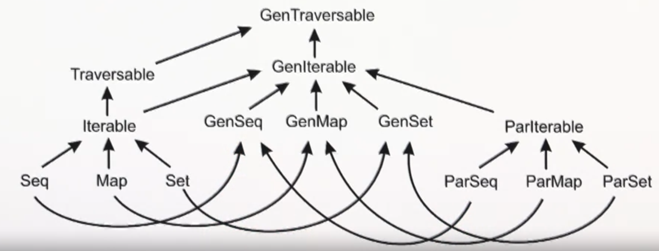
Scala collections hierarchy

Traversable[T] - collection of elements with operations implemented using foreach
Iterable[T] - subtype of Traversable, operations implemented using iterator
Seq[T] - ordered sequence
Set[T] - set of non duplicates
Map[K, V] - map of keys and values

Their parallel counterparts are ParIterable, ParSeq, ParSet, and ParMap

For code agnostic about parallelism, there is a separate hierarchy of generic collection traits: GenIterable, GenSeq, GenSet, GenMap. Generic collections can be used as parameters in functions, where we can then pass either a sequential or parallel collections

Collections hierarchy

The Iterator

trait Iterator[A] {
  def next(): A
  def hasNext: Boolean
  def foldLeft[S](z: S)(f: (S, T) => S): S = {
    var result = z
    while (hasNext) result = f(result, next())
    result
  }

}

The Splitter

A Splitter is a special case of an Iterator and helps to partition a collection into multiple disjoint subsets. The idea is that after the splitting, these subsets can be processed in parallel. You can obtain a Splitter from a parallel collection by invoking .splitter on it

To split a Splitter, simply use .split, which returns Seq[Splitter[A]], the sequence of new splitters, each containing a subset of the collection. Each Splitter has an attribute remaining: the number of elements of the current collection. remaining can be used as a threshold value (to split or stop splitting)

The Builder

Builders are used internally to create new (sequential) collections. Here is an example of filter using a Builder. Repr == Seq[T]

trait Builder[A, Repr] {
  def +=(elem: A): Builder[A, Repr]
  def result: Repr
}

def newBuilder: Builder[A, Repr]

def filter(predicate: T => Boolean): Repr = {
  val b = newBuilder
  for (x <- this) if (predicate(x)) b += x
  b.result
}

The Combiner

A Combiner is a parallel version of a Builder, and a counterpart to a Splitter

trait Combiner[T, Repr] extends Builder [T, Repr] {
  def combine(that: Combiner[T, Repr]): Combiner[T, Repr]
}

Converting (parallelizing) collections

Arrays, Ranges, Vectors, HashSets, HashMaps and TrieMaps can be converted to parallel by using the par method

List is converted to a parallel vector. Pick parallelizable data structures such as Vector in favour of non parallelizable, such as List

Thread safe collections

ConcurrentSkipListSet and ConcurrentSkipListMap are useful when you need a sorted container that will be accessed by multiple threads. These are essentially the equivalents of TreeMap and TreeSet for concurrent code (source: StackOverflow)

Never write to a collection that is concurrently traversed
Neved read from a collection that is concurrently modified

TrieMap collection and snapshot

The TrieMap is an exception to the above rules. The snapshot method can be used to efficiently grab (clone) its current state, avoid concurrent modifications of a traversed collection

Parallel fold?

Although we can't use reduce or foldLeft in parallel, it is possible to use fold in parallel. fold has a nicer type signature with a neutral element, which allows for data parallelism when using associative functions, where the neutral element and the functions share a common type:

xs.par.fold(0)(_ + ) // parallel sum a xs
xs.par.fold(Int.MinValue)(math.max)

To ensure fold works correctly under parallel cases, the neutral element and the binary operator must form a monoid

Aggregate

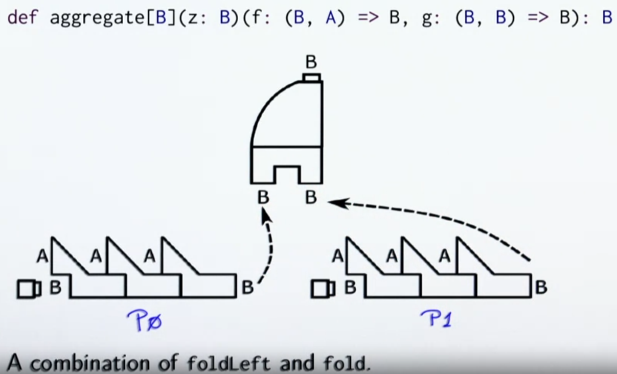
alt Aggregate has a neutral element, a folding operator, and a parallel grouping operator

// count vowels
Array('E', 'P', 'F', 'L').par.aggregate(0)(
  (count, c) => if (isVowel(c)) count + 1 else count, // folding operator
  _ + _  // grouping operator
)

Implementing Combiners

Combine means union or concatenation depending on the data structure. The combine method must be efficient, executing in O(log n + log m) time, where n and m are the sizes of two input combiners

Arrays CANNOT be efficiently concatenated. Most set implementations do not have efficient union

Parallel two-phase construction

When using combiners, the intermediate data structures are of the same type that the final data structure

In two-phase construction, the intermediate data structure is a different one, having an efficient combine method, and an efficient += method

The two phases are:

Combine the intermediate data structures until there is only one of them
Transform the only data structure left to the desired type

Efficient two-phase construction of arrays is based on nested array buffers and pointer (reference) copying

Efficient two-phase construction of hash tables is based on buckets containing a linked list of arrays, non-overlapping based on a hashcode

Efficient two-phase construction of search trees is based on total ordering and non-overlapping intervals

Conc-tree data structure

Trees are only good for parallelism if they are balanced. For that, we have a data type called Conc, which represents balanced trees

sealed trait Conc[+T] {
  def level: Int
  def size: Int
  def left: Conc[T]
  def right: Conc[T]
}

case object Empty extends Conc[Nothing] {
  def level = 0
  def size = 0
}

class Single[T](val x: T) extends Conc[T] {
  def level = 0
  def size = 1
}

case class <>[T](left: Conc[T], right: Conc[T]) extends Conc[T] {
  val level = 1 + math.max(left.level, right.level)
  val size = left.size + right.size
}

The level difference between the left and right subtree of a <> must be 1 or less

Amortized, constant-time append operation

def +=(elem: T) {
  xs = xs <> Single(elem)
}

case class Append[T](left: Conc[T], right: Conc[T]) extends Conc[T] ...

Append trees has O(1) append and O(log n) concatenation